Summary

E-scooters overran Portland during the pilot period during summer 2018, and gave rise to a new gig-economy role: finding scooters scattered around town to charge nightly. In this post, I build and explore a genetic algorithm to efficiently find good routing solutions to this TSP problem and a TSP-like problem (with qualitatively different behavior) if the solution-space is constrained.

Introduction

Last summer in Portland we had an e-scooter pilot program, and people (nicknamed juicers) were paid by the scooter operators to pick up scooters with low battery and charge them. These scooters were available for pickup after 9, and there was often fierce competition to be the one getting to them (e.g., see here: https://www.wweek.com/news/2018/08/07/i-signed-on-to-portlands-latest-side-hustle-collecting-electric-scooters-and-charging-them-at-night/). Assuming that not every scooter can be picked up by one user, the task for a juicer is to pick up as many as possible and find the most efficient route between them. If length of time is not a constraint, or there aren’t any other people trying to pick up scooters, the problem is the TSP; with shift length, the problem is finding the largest-possible subset of scooters for which the TSP solution is shorter than the shift length. This problem has analogues with dockless bikeshare, for example: bikes need monthly inspections and maintenance, and not all bikes needing care be visited in one shift.

The Traveling Salesperson Problem (TSP) is a classic problem in combinatoric optimization: given a set of nodes (cities, customers, scooters), find the shortest path that visits them all once. The TSP comes in many flavors, according to various real-world operations constraints: customers may need to be visited in specific time intervals, or there may be multiple vehicles to route, for example.

This TSP and its variants are NP-hard problems, meaning that no efficient method for finding the optimal solution exists: even for problems of size 30, heuristics need to be used as the solution space is so large it’s impossible to search every possible solution. Heuristics used for the TSP include tabu search, simulated annealing, ant colony optimization, and genetic algorithms. Inspired by a class on Artificial Life I took during Fall 2018, I built a genetic algorithm (GA) from scratch in Python for this problem.

Genetic Algorithms

Genetic algorithms were first invented in 1975 by John Holland, and rely on processes similar to biological natural selection. The process efficiently searches the solution space and identifies ‘good’ solutions. These good solutions are more likely to be selected in the next generation, so generally there is a selective pressure for better and better solutions. GAs start with a diverse population of solutions, and then operators such as crossover and mutations are used to alter the offspring solutions.

It had been a while since I used object-oriented programming, so I wanted to refresh my skills by building classes. I defined two classes: an Algorithm class and an Environment class. The Algorithm solution is an array of length n + 2, where each n_i is the ID of the scooter to visit. The route is read linearly left-to-right. The first and last element are fixed, forcing the solution to return to the place it began. However, the length of the solution can vary: the shortest solution would have length n = 2, where no scooters are visited, and the longest solution would have length N + 2, where N is the total number of scooters. However, the fitness of a solution is the number of scooters it visits, so longer solutions are favored.

The length and order of an individual solution is fixed, but offspring algorithms can have genes inverted (re-ordered), mutated (swapping the position of two genes, or swapping with a scooter not already visited), or added. Genes are also rearranged when creating a child solution from two parent solutions. Apart from the gene addition, inversion, mutation, and recombination are classic GA operators that increase diversity (and therefore increase the number of solutions visited within the search space). If the environment imposes constraints (i.e., a maximum solution time length or distance for the juicer), feasibility of the child solution is assessed. Only feasible solutions are kept.

The Environment class is responsible for defining which scooters are available and the locations of them. It initializes a population of algorithms, selects the best, and then iterates until the maximum nuber of iterations or time interval is reached.

Results

There are two qualitatively different patterns of behavior, depending on if the solutions are constrained or unconstrained. As mentioned above, the unconstrained problem is exactly the TSP: all scooters are visited, and the best solution is the shortest one between them.

Unconstrained

When the distance is unconstrained, the best GA solutions visit every scooter, and tries to optimize the TSP. As seen in the image below, in the first generation (iteration), even the best-looking solution doesn’t look great. Over the generations, however, the route starts looking more and more reasonable – and the distance traveled by the best solution decreases too.

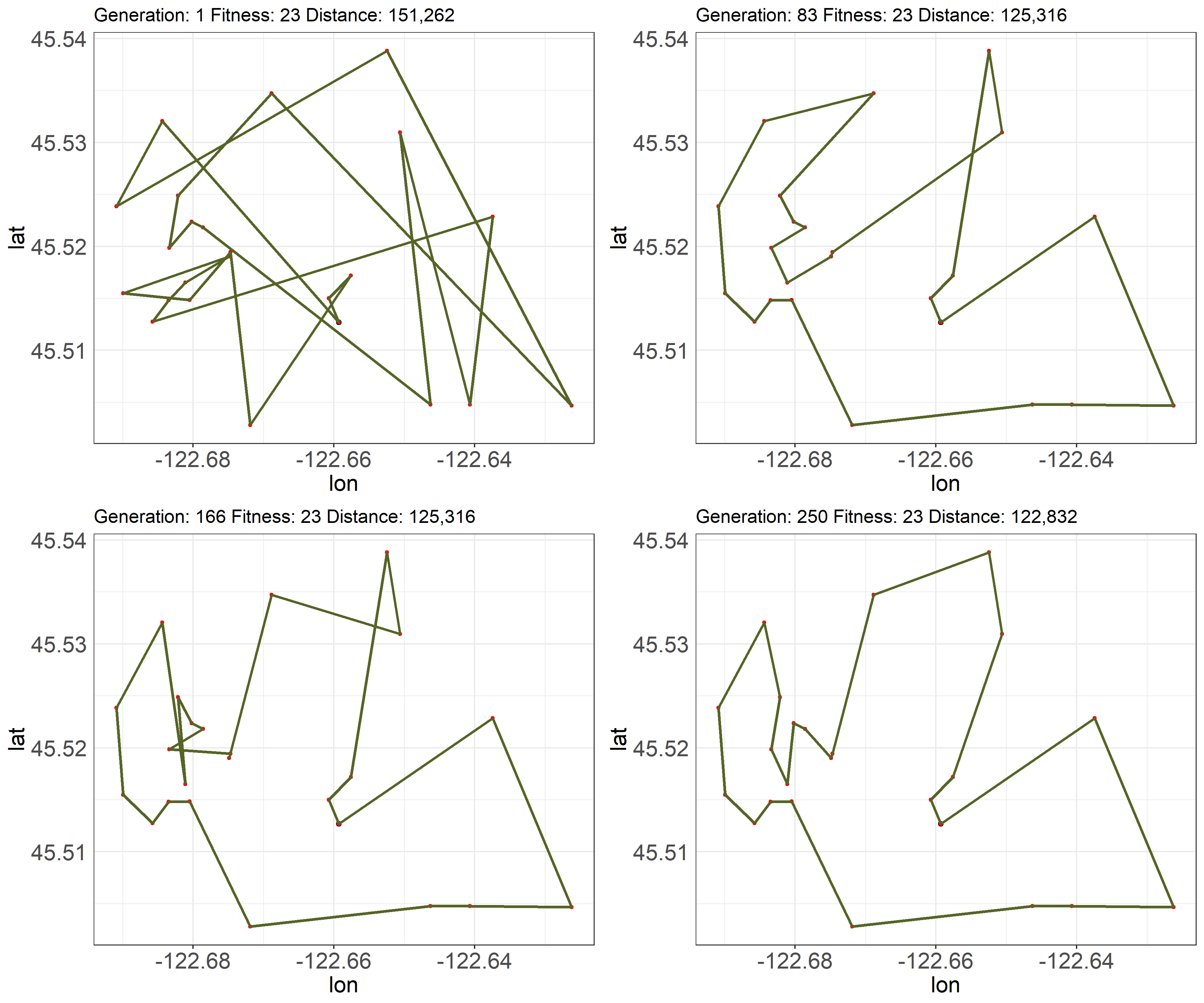
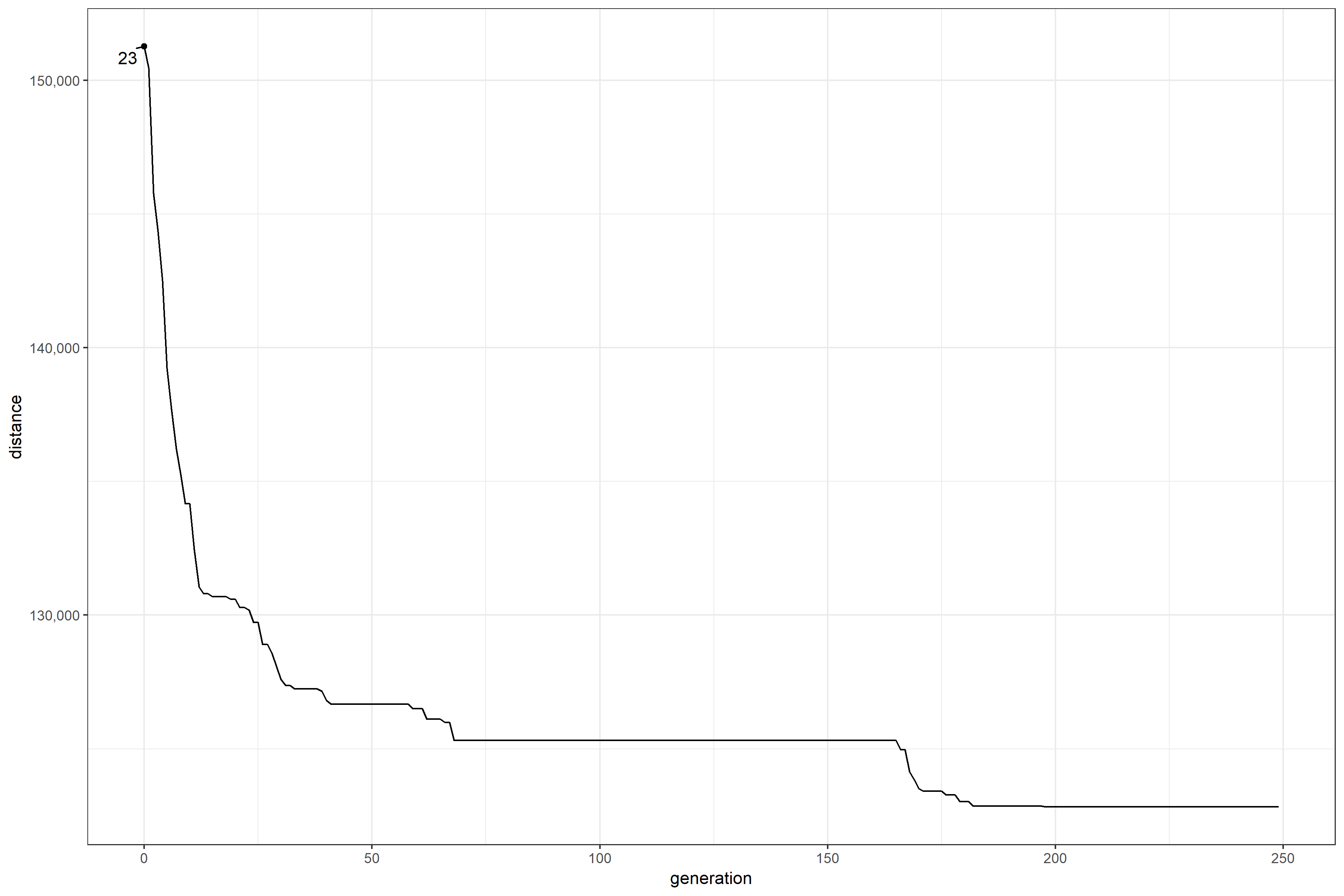
An alternate way of visualizing these results is below. It displays the distance traveled by the best solution at each generation. The 23 annotating the point displays the number of scooters visited. The distance falls monotonically, quickly at first and then plateauing. Around generation 180, the solution flatlines and doesn’t change. It looks like an optimal solution has been found.

Constrained

When the distance is constrained, even the best solutions may not visit every scooter. Instead, the GAs try to fit in as many scooters as possible within the distance limit. In the image shown below, scooters are red, and the route between them is in green. Not all scooters are visited (there isn’t a green line connecting every red dot). As in the unconstrained case, the first generation is pretty bad at finding a good solution: it visits only 27 scooters with the total distance traveled at 175,000 meters. Over the generations, the number of scooters increases, and the solution starts looking more and more reasonable. There isn’t much in the final solution that looks like it could be changed without going over the distance limit.

The alternate way of showing the distance traveled shows some interesting behavior. The distance traveled stays within 165,000 to 175,000 meters. Adding a new scooter is represented by a new number on the point: the first generation’s best solution visits 27 scooters, and a few generations later it increases to 28, 29, and further. Generally adding a scooter to the solution increases the distance traveled, but then falls as a more efficient route is found (or a different scooter is swapped in). The final solution, which visits 36 scooters, stays quite stable after roughly 100 generations.

Conclusion

This work shows that GAs can efficiently find good solutions to a routing problem, both with constrained and unconstrained distances. When the distance is unconstrained, the problem is the Traveling Salesman Problem. When distance is constrained, the problem is finding the most nodes (scooters) that can be visited within the distance limit. Even though the scooter pilot program is over in Portland, this methodology has applications in bikeshare (routing to visit broken bikes or bikes needing inspection), and other routing problems within operations.